 Data
Mining - Bayesian Approaches
Data
Mining - Bayesian Approaches
Data
Mining - Bayesian Approaches
|
Data Mining Course [CISC 873, School of Computing, Queen's University] |
|
Bayesian Approaches Tutorials and Applying Results [Henry 2004] |
Data Mining (DM)
Introduction
DM Definitions
DM Web Pages
Bayesian Tutorials
Overview
Naïve Bayesian Classifiers
Gaussian Bayesian Classifiers
Bayesian Networks
Applying Bayesian Approach
on Datasets
Dataset #1
Dataset #2
Dataset #3
Dataset
Additional
Mining Software
Weka
MatLab
| Resource | Define |
| Two Crows | An information extraction activity whose goal is to discover hidden facts contained in databases. Using a combination of machine learning, statistical analysis, modeling techniques and database technology, data mining finds patterns and subtle relationships in data and infers rules that allow the prediction of future results. Typical applications include market segmentation, customer profiling, fraud detection, evaluation of retail promotions, and credit risk analysis. |
| Gotcha | A type of application with built-in proprietary algorithms that sort, rank, and perform calculations on a specified and often large data set, producing visualizations that reveal patterns which may not have been evident from mere listings or summaries. |
| The OLAP Report | The process of using statistical techniques to discover subtle relationships between data items, and the construction of predictive models based on them. The process is not the same as just using an OLAP tool to find exceptional items. Generally, data mining is a very different and more specialist application than OLAP, and uses different tools from different vendors. Normally the users are different, too. |
Data Mining Web Pages:
Statistical Data Mining Tutorials (by Andrew Moore) - Highly recommended! Excellent introductions to the DM techniques.
An Introduction Student Notes - Good materials to accompany with the course.
An Introduction to Data Mining (by Kurt Thearling) - General ideas of why we need to do DM and how DM works.
The Data Mine - Launched in April 1994, and providing information about DM. Nice place to find topics in DM.
CISC873 Data Mining - Finally, our course page which is obvious necessary here.
[To Index]
Bayesian approaches are a fundamentally important DM technique. Given the probability distribution, Bayes classifier can provably achieve the optimal result. Bayesian method is based on the probability theory. Bayes Rule is applied here to calculate the posterior from the prior and the likelihood, because the later two is generally easier to be calculated from a probability model.
One limitation that the Bayesian approaches can not cross is the need of the probability estimation from the training dataset. It is noticeable that in some situations, such as the decision is clearly based on certain criteria, or the dataset has high degree of randomality, the Bayesian approaches will not be a good choice.
My introduction slides of Bayesian Approaches. [pdf]
The Naïve Bayes Classifier technique is particularly suited when the dimensionality of the inputs is high. Despite its simplicity, Naive Bayes can often outperform more sophisticated classification methods. The following example is a simple demonstration of applying the Naïve Bayes Classifier from StatSoft.
As
indicated at Figure 1, the objects can be classified as either GREEN or RED. Our
task is to classify new cases as they arrive (i.e., decide to which class label
they belong, based on the currently exiting objects).
 Figure
1. objects are classified to GREEN or RED.
Figure
1. objects are classified to GREEN or RED.
We can then calculate the priors (i.e. the probability of the object among all objects) based on the previous experience. Thus:
Since there is a total of 60 objects, 40 of which are GREEN and 20 RED, our prior probabilities for class membership are:
Having formulated our prior probability, we are now ready to classify a new object (WHITE circle in Figure 2). Since the objects are well clustered, it is reasonable to assume that the more GREEN (or RED) objects in the vicinity of X, the more likely that the new cases belong to that particular color. To measure this likelihood, we draw a circle around X which encompasses a number (to be chosen a priori) of points irrespective of their class labels. Then we calculate the number of points in the circle belonging to each class label.
 Figure
2. classify the WHITE circle.
Figure
2. classify the WHITE circle.
We can calculate the likelihood:
In Figure 2, it is clear that Likelihood of X given RED is larger than Likelihood of X given GREEN, since the circle encompasses 1 GREEN object and 3 RED ones. Thus:
Although the prior probabilities indicate that X may belong to GREEN (given that there are twice as many GREEN compared to RED) the likelihood indicates otherwise; that the class membership of X is RED (given that there are more RED objects in the vicinity of X than GREEN). In the Bayesian analysis, the final classification is produced by combining both sources of information (i.e. the prior and the likelihood) to form a posterior probability using Bayes Rule.
Finally, we classify X as RED since its class membership achieves the largest posterior probability.
[To Index]
The problem with the Naïve Bayes Classifier is that it assumes all attributes are independent of each other which in general can not be applied. Gaussian PDF can be plug-in here to estimate the attribute probability density function (PDF). Because the well developed Gaussian PDF theories, we can classify the new object easier through the same Bayes Classifier Model but with certain degree recognition of the covariance. Normally, this gives more accurate classification result.
I guess one question to be asked is why Gaussian? There are many other PDF's can be applied. But from statistic point of view, many real world distributions are more likely to be estimated by Gaussian PDF than others. If you are familiar with Information Theory, the Gaussian gives the maximum entropy for an unbounded range, which means Gaussian has more ability to estimate the randomality.
How to apply the Gaussian to the Bayes Classifier?
The application here is very intuitive. We assume the Density Estimation follows a Gaussian distribution. Then the prior and the likelihood can be calculated through the Gaussian PDF. The critical thing here is to identify the Gaussian distribution (i.e. find the mean and variance of the Gaussian). The following 5 steps are a general model to initialize the Gaussian distribution to fit our input dataset.
Choose a probability estimator form (Gaussian)
Choose an initial set of parameters for the estimator (Gaussian mean and variance)
Given parameters, compute posterior estimates for hidden variable
Given posterior estimates, find distributional parameters that maximize expectation (mean) of joint density for data and hidden variable (Guarantee to also maximize improvement of likelihood)
Assess goodness of fit (i.e. log likelihood) If not stopping criterion, return to (3).
From research perspective, Gaussian may not be the only PDF to be applied to the Bayes Classifier, although it has very strong theoretical support and nice properties. The general model of applying those PDF's should be the same. The estimation results highly depend on whether or how close a PDF can simulate the given dataset.
Some normal used PDF's are listed below: (just to refresh our statics)
[To Index]
First of all, there is a nice introduction to Bayesian Networks and their Contemporary Applications by Daryle Niedermayer [web page]. It is generally hard for me to come up with a better one here. So the following may just a simpler version of Daryle's introduction.
From the previous tutorial on Gaussian Bayes Classifier, we notice that the Gaussian model helps to integrate some correlation which improves the classification performance against the Naïve model assuming the independence. However, using Gaussian model with Bayes Classifier still has its limitation of generating the correlations. So it is where the Bayesian Networks (Bayes Nets) get involved.
Bayes Net is a model of utilizing the conditional probabilities among different variables. It is generally impossible to generate all conditional probabilities from a given dataset. Our task is to pick important ones and use them in the classification process. So essentially, a Bayes net is a set of "Generalized Probability Density Function" (gpdf).
Informally, we can define a Bayes net as an augmented directed acyclic graph, represented by the vertex set V and directed edge set E. Each vertex from V represents an attribute, and each edge from E represents a correlation between two attributes. One example of five attributes Bayes net is shown in Figure 3.
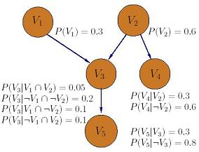 Figure 3. A Bayes net for 5 attributes.
Some important observations here:
There is no loop in the graph representation since it is acyclic.
Two variable vi and vj may still correlated even if they are not connected.
Each variable vi is conditionally independent of all non-descendants, given its parents.
Now, let's suffer the mathematical definition formally.
Consider a domain U of n variables, x1,...xn.
Each variable may be discrete having a finite or countable number of
states, or continuous. Given a subset X of variables xi where
xi
![]() U, if one can observe the state of every variable in X, then this observation is
called an instance of X and is denoted as X=
U, if one can observe the state of every variable in X, then this observation is
called an instance of X and is denoted as X=![]() for the observations
for the observations
![]() . The
"joint space" of U is the set of all instances of U.
. The
"joint space" of U is the set of all instances of U.
![]() denotes
the "generalized probability density" that X=
denotes
the "generalized probability density" that X=![]() given Y=
given Y=![]() for a person with current state information
for a person with current state information
![]() . p(X|Y,
. p(X|Y,
![]() ) then
denotes the gpdf for X, given all possible observations of Y. The
joint gpdf over U is the gpdf for U.
) then
denotes the gpdf for X, given all possible observations of Y. The
joint gpdf over U is the gpdf for U.
A Bayesian network for domain U
represents a joint gpdf over U. This representation consists of a set of
local conditional gpdfs combined with a set of conditional independence
assertions that allow the construction of a global gpdf from the local
gpdfs. Then these value can be ascertained as:
![]() (Equation
1)
(Equation
1)
A Bayesian Network Structure then encodes the assertions of conditional independence in Equation 1 above. Essentially then, a Bayesian Network Structure Bs is a directed acyclic graph such that (1) each variable in U corresponds to a node in Bs, and (2) the parents of the node corresponding to xi are the nodes corresponding to the variables in [Pi]i.
It is not hard to argue the advantage of using Bayes net model here. But formal analysis needs to be done with the probability inference theory which we have briefly discussed in the next section. For reader who is not interested with the analysis mathematically, ignore the next section to avoid confusion (sometimes not bad).
How to build a Bayes Net? A general model can be followed below:
Choose a set of relevant variables.
Choose an ordering for the variables.
Assume the variables are X1, X2, ..., Xn (where X1 is the first, and Xi is the ith).
for i = 1 to n:
Add the Xi vertex to the network
Set Parent(Xi) to be a minimal subset of X1, ..., Xi-1, such that we have conditional independence of Xi and all other members of X1, ..., Xi-1 given Parents(Xi).
Define the probability table of P(Xi=k | Assignments of Parent(Xi)).
There are many choices of how to select relevant variables, as well as how to estimate the conditional probabilities. If we imagine the network as a connection of Bayes classifiers, then the probability estimation can be done applying some PDF like Gaussian. In some cases, the design of the network can be rather complicated. There are some efficient ways of getting relevant variables from the dataset attributes. Assume the coming signal to be stochastic will give a nice way of extracting the signal attributes. And normally, the likelihood weighting is another way to getting attributes.
[To Index]
Applying Bayesian Approach on Datasets
Dataset Preliminary Analysis [pdf]
Attribute Selection results:
CfsSubsetEval with BestFirst (15 attributes)[txt]
InfoGainAttibuteEval with Ranker (12 attributes 0.1000 above) [txt]
ClassifierSubsetEval (NaiveBayes) with BestFirst (11 attributes) [txt]
ClassifierSubsetEval (BayesNet) with BestFirst [txt]
Preliminary Mining results (selected):
All attributes with NaiveBayes (82% training) [txt]
- 80 %
15 attributes (CfsSubsetEval) with AODE (82% training) [txt]
- 84 %
12 attributes (InfoGainAttributeEval) with BayesNets (82% training) [txt]
- 84 %
11 attributes with (ClassifierSubsetEval-NaiveBayes) BayesNets (65%
training) [txt] - 87.7551%
12 attributes with (ClassifierSubsetEval-BayesNet) BayeNets (78% training) [txt]
- 87.0968 %
Record "optimal" result:
12 attributes (InfoGainAttributeEval) with AODE (82% training) [txt] - 92%
Attribute subsets:
CfsSubesetEval -------------------------- {10, 11, 14, 24, 25, 27, 65, 71, 74,
83, 88, 92, 107, 115, 119}
InfoGainAttributeEval ------------------- {11, 15, 19, 24, 27, 29, 71, 81, 88,
92, 115, 119}
ClassifierSubsetEval(NaiveBayes) - { 6, 9, 10, 19, 24, 49, 59, 65,
72, 100, 115}
ClassifierSubsetEval(BayesNet) ---- { 7, 10, 28, 37, 46, 49, 57, 64, 81,
88, 91, 115}
What are the "important" attributes?
*Please note that the attribute order is different from the original .csv file. We removed the 6 attributes and dicretized all attributes. Please use the file here to see the order.
Mining Results [pdf]
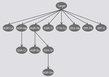
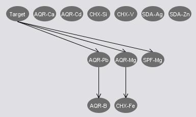
We mainly look at the Bayes Net in our final mining process since the Bayes network demonstrates some statistic properties like the independence and inference, which may be helpful for us to select attributes. Some Bayes networks which are built by Weka using the attribute sets from the preliminary analysis are shown below.
|
|
|
|
InfoGainArributeEval Set (12) |
ClassifierSubsetEval(NaiveBayes) (11) |
|
|
|
|
ClassifierSubsetEval(BayesNet) (12) |
|
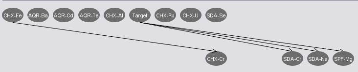
The attribute set from the InfoGainArributeEval has more correlations from the generated network. This may or may not be a good news to the Bayes Net since some correlation may distract the classification process. The attribute sets from both ClassifierSubsetEval(NaiveBayes) and ClassifierSubsetEval(BayesNet) have some independences between the "target" attribute and other attributes. We consider to remove those attributes that are independent to "target" since they are in some degree irrelevant towards our classification. We further tried to combine the two sets' "target" correlated attributes, and got a set of 8 attributes as listed below.
Combined Attribute Set: {AQR-B, AQR-Mg, AQR-Pb, CHX-Fe, SDA-Cr, SDA-Na, SDA-Se, SPF-Mg}
The Bayes network constructed by Weka is showed in below figure, and the classification result is here [txt].
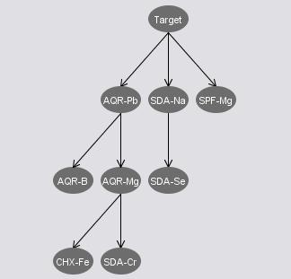
The training and testing split is at 66%, and we can see from the network that all attributes are correlated. Some result discussion is proposed in the first dataset mining result slide.
Finally, here is a nice Bayes Net Weka description by the developer just came out this September. [pdf]
We plot some attributes against the AMGN attribute, and it does look like forming some clusters. However, we have not figure out how to employ this to improve our mining result. [pdf] (plot)
[To Index]
Dataset Preliminary Analysis [pdf]
Microarray Data Cleaning
We remove the "Gene Description" column first, and change the "Gene Accession Number" to "ID".
We normalize the data such that for each value, set the minimum field value to 20 and the maximum to 16,000. (i.e. the expression values less than 20 or over 16,000 were considered by biologists as unreliable for this experiment.).
We transpose the data making each column representing an attribute and each row representing a record. (i.e. the data transpose is needed to get the CSV file compatible with Weka. The transpose is done by MatLab.)
We further add a "Class" attribute to indicate the kind of leukemia. (i.e. Class {ALL, AML})
The cleaned training data can be downloaded here [csv].
Some internet tip suggests to remove the initial records with Gene Description
containing "control)".
(Those are Affymetrix controls, not human genes), which has not been applied in
our cleaning steps.
Attribute Selection / Feature Reduction
There are in total 7070 genes (attributes) in the dataset. It is critical to do the attribute selection. We take the standard Signal to Noise (S2N) ratio and T-value to get significant attribute set. (Note that it is impractical to run any attribute selection algorithm from Weka since the memory requirement would be huge.)
Let Avg1, Avg2 be the average expression values.
Let Stdev1,
Stdev2 be the sample standard deviations.
S2N = (Avg1 - Avg2)/(Stdev1 + Stdev2)
T-value = (Avg1 - Avg2)/sqrt(Stdev1*Stdev1/N1+Stdev2*Stdev2/N2)
Where N1 is
the number of ALL observations, and N2 is the number of AML observations.
T-value
T-value is the observed value of the T-statistic that is used to test the
hypothesis that two attributes are correlated. The T-value can range between
-infinity and +infinity. A T-value near 0 is evidence for the null hypothesis
that there is no correlation between the attributes. A T-value far from 0
(either positive or negative) is evidence for the alternative hypothesis that
there is correlation between the attributes.
Top 50 genes with the highest S2N ratio:
|
Rank |
Gene Name |
S2N |
T-value |
|
Rank |
Gene Name |
S2N |
T-value |
|
1 |
M55150_at |
1.467641 |
8.091951 |
26 |
L08246_at |
1.034784 |
4.506267 |
|
|
2 |
X95735_at |
1.444531 |
5.727643 |
27 |
X74262_at |
1.027773 |
6.016389 |
|
|
3 |
U50136_rna1_at |
1.421708 |
6.435952 |
28 |
M62762_at |
1.023393 |
5.122153 |
|
|
4 |
U22376_cds2_s_at |
1.339308 |
7.9043 |
29 |
M31211_s_at |
1.022881 |
6.294207 |
|
|
5 |
M81933_at |
1.204042 |
6.164965 |
30 |
M28130_rna1_s_at |
1.001286 |
3.911006 |
|
|
6 |
M16038_at |
1.203218 |
4.930437 |
31 |
D26156_s_at |
0.989098 |
6.097113 |
|
|
7 |
M84526_at |
1.20142 |
4.057042 |
32 |
M63138_at |
0.983628 |
4.048325 |
|
|
8 |
M23197_at |
1.195974 |
4.737778 |
33 |
M31523_at |
0.971228 |
5.677543 |
|
|
9 |
U82759_at |
1.192556 |
6.24302 |
34 |
M57710_at |
0.967686 |
3.69931 |
|
|
10 |
Y12670_at |
1.184737 |
5.324928 |
35 |
X15949_at |
0.96009 |
5.389656 |
|
|
11 |
D49950_at |
1.143704 |
5.588063 |
36 |
M69043_at |
0.95886 |
4.708053 |
|
|
12 |
M27891_at |
1.133427 |
3.986204 |
37 |
S50223_at |
0.956733 |
5.858626 |
|
|
13 |
X59417_at |
1.124637 |
6.803106 |
38 |
U32944_at |
0.954875 |
5.442992 |
|
|
14 |
X52142_at |
1.122589 |
5.833144 |
39 |
M81695_s_at |
0.953066 |
4.195556 |
|
|
15 |
M28170_at |
1.116756 |
6.253971 |
40 |
L47738_at |
0.95138 |
5.715039 |
|
|
16 |
X17042_at |
1.105975 |
5.388623 |
41 |
M83652_s_at |
0.947504 |
3.721478 |
|
|
17 |
U05259_rna1_at |
1.103966 |
6.175126 |
42 |
X85116_rna1_s_at |
0.946372 |
3.923369 |
|
|
18 |
Y00787_s_at |
1.081995 |
4.701085 |
43 |
M11147_at |
0.945755 |
5.588645 |
|
|
19 |
M96326_rna1_at |
1.07719 |
3.869518 |
44 |
Z15115_at |
0.9452 |
5.615471 |
|
|
20 |
U12471_cds1_at |
1.069731 |
6.146299 |
45 |
M21551_rna1_at |
0.941981 |
5.377292 |
|
|
21 |
U46751_at |
1.064078 |
4.127982 |
46 |
M19045_f_at |
0.938076 |
3.834549 |
|
|
22 |
M80254_at |
1.044395 |
4.271131 |
47 |
X04085_rna1_at |
0.930499 |
4.931191 |
|
|
23 |
M92287_at |
1.043056 |
6.217365 |
48 |
L49229_f_at |
0.920745 |
5.398203 |
|
|
24 |
L13278_at |
1.042032 |
6.021342 |
49 |
X14008_rna1_f_at |
0.914954 |
3.655554 |
|
|
25 |
U09087_s_at |
1.036257 |
6.182425 |
50 |
M91432_at |
0.913521 |
5.300882 |
The S2N training dataset (50 top genes) can be downloaded here [csv]
(transposed).
The S2N testing dataset (50 top genes) can be downloaded here [csv]
(transposed).
Top 50 genes with the highest T-value:
|
Rank |
Gene Name |
S2N |
T-value |
|
Rank |
Gene Name |
S2N |
T-value |
|
1 |
M55150_at |
1.467641 |
8.091951 |
26 |
U32944_at |
0.954875 |
5.442992 |
|
|
2 |
U22376_cds2_s_at |
1.339308 |
7.9043 |
27 |
U26266_s_at |
0.887813 |
5.425205 |
|
|
3 |
X59417_at |
1.124637 |
6.803106 |
28 |
J05243_at |
0.886777 |
5.406254 |
|
|
4 |
U50136_rna1_at |
1.421708 |
6.435952 |
29 |
L49229_f_at |
0.920745 |
5.398203 |
|
|
5 |
M31211_s_at |
1.022881 |
6.294207 |
30 |
X15949_at |
0.96009 |
5.389656 |
|
|
6 |
M28170_at |
1.116756 |
6.253971 |
31 |
X17042_at |
1.105975 |
5.388623 |
|
|
7 |
U82759_at |
1.192556 |
6.24302 |
32 |
M21551_rna1_at |
0.941981 |
5.377292 |
|
|
8 |
M92287_at |
1.043056 |
6.217365 |
33 |
M31303_rna1_at |
0.875318 |
5.370571 |
|
|
9 |
U09087_s_at |
1.036257 |
6.182425 |
34 |
Y08612_at |
0.877482 |
5.366653 |
|
|
10 |
U05259_rna1_at |
1.103966 |
6.175126 |
35 |
U20998_at |
0.896103 |
5.361239 |
|
|
11 |
M81933_at |
1.204042 |
6.164965 |
36 |
AF012024_s_at |
0.873658 |
5.333337 |
|
|
12 |
U12471_cds1_at |
1.069731 |
6.146299 |
37 |
X56411_rna1_at |
0.870983 |
5.327392 |
|
|
13 |
D26156_s_at |
0.989098 |
6.097113 |
38 |
Y12670_at |
1.184737 |
5.324928 |
|
|
14 |
L13278_at |
1.042032 |
6.021342 |
39 |
U29175_at |
0.908033 |
5.322716 |
|
|
15 |
X74262_at |
1.027773 |
6.016389 |
40 |
M91432_at |
0.913521 |
5.300882 |
|
|
16 |
S50223_at |
0.956733 |
5.858626 |
41 |
HG1612-HT1612_at |
0.856338 |
5.276869 |
|
|
17 |
X52142_at |
1.122589 |
5.833144 |
42 |
M13792_at |
0.866312 |
5.222356 |
|
|
18 |
X95735_at |
1.444531 |
5.727643 |
43 |
D63874_at |
0.844716 |
5.206861 |
|
|
19 |
L47738_at |
0.95138 |
5.715039 |
44 |
U72342_at |
0.848128 |
5.206761 |
|
|
20 |
M31523_at |
0.971228 |
5.677543 |
45 |
X97267_rna1_s_at |
0.844922 |
5.203003 |
|
|
21 |
Z15115_at |
0.9452 |
5.615471 |
46 |
X76648_at |
0.861562 |
5.195203 |
|
|
22 |
M11147_at |
0.945755 |
5.588645 |
47 |
U35451_at |
0.842047 |
5.144391 |
|
|
23 |
D49950_at |
1.143704 |
5.588063 |
48 |
Z69881_at |
0.896518 |
5.143816 |
|
|
24 |
X63469_at |
0.905744 |
5.583296 |
49 |
D63880_at |
0.833577 |
5.125102 |
|
|
25 |
D38073_at |
0.902946 |
5.562983 |
50 |
M62762_at |
1.023393 |
5.122153 |
The T-value training dataset (50 top genes) can be downloaded here [csv]
(transposed).
The T-value testing dataset (50 top genes) can be downloaded here [csv]
(transposed).
Common genes from the above two sets:
31 attributes in the common set: {D26156_s_at, D49950_at, L13278_at, L47738_at, L49229_f_at, M11147_at, M21551_rna1_at, M28170_at, M31211_s_at, M31523_at, M55150_at, M62762_at, M81933_at, M91432_at, M92287_at, S50223_at, U05259_rna1_at, U09087_s_at, U12471_cds1_at, U22376_cds2_s_at, U32944_at, U50136_rna1_at, U82759_at, X15949_at, X17042_at, X52142_at, X59417_at, X74262_at, X95735_at, Y12670_at, Z15115_at}
Common set attributes can be visualized here.
From statistic aspect, the common attribute set contains those attributes that
have high discriminating ability to distinguish ALL and AML leukemia.
The Common training dataset (31 common genes) can be downloaded here [csv]
(transposed).
The Common testing dataset (31 common genes) can be downloaded here [csv]
(transposed).
Preliminary result with NaiveBayes and BayesNet
|
ID |
NB(S2N) |
BN(S2N) |
NB(T) |
BN(T) |
NB( C) |
BN( C) |
|
39 |
ALL |
ALL |
ALL |
ALL |
ALL |
ALL |
|
40 |
ALL |
ALL |
ALL |
ALL |
ALL |
ALL |
|
42 |
ALL |
ALL |
ALL |
ALL |
ALL |
ALL |
|
47 |
ALL |
ALL |
ALL |
ALL |
ALL |
ALL |
|
48 |
ALL |
ALL |
ALL |
ALL |
ALL |
ALL |
|
49 |
ALL |
ALL |
ALL |
ALL |
ALL |
ALL |
|
41 |
ALL |
ALL |
ALL |
ALL |
ALL |
ALL |
|
43 |
ALL |
ALL |
ALL |
ALL |
ALL |
ALL |
|
44 |
ALL |
ALL |
ALL |
ALL |
ALL |
ALL |
|
45 |
ALL |
ALL |
ALL |
ALL |
ALL |
ALL |
|
46 |
ALL |
ALL |
ALL |
ALL |
ALL |
ALL |
|
70 |
ALL |
ALL |
ALL |
ALL |
ALL |
ALL |
|
71 |
ALL |
ALL |
ALL |
ALL |
ALL |
ALL |
|
72 |
ALL |
ALL |
ALL |
ALL |
ALL |
ALL |
|
68 |
ALL |
ALL |
ALL |
ALL |
ALL |
ALL |
|
69 |
ALL |
ALL |
ALL |
ALL |
ALL |
ALL |
|
67 |
AML |
AML |
ALL |
ALL |
AML |
AML |
|
55 |
ALL |
ALL |
ALL |
ALL |
ALL |
ALL |
|
56 |
ALL |
ALL |
ALL |
ALL |
ALL |
ALL |
|
59 |
ALL |
ALL |
ALL |
ALL |
ALL |
ALL |
|
52 |
AML |
AML |
AML |
AML |
AML |
AML |
|
53 |
AML |
AML |
AML |
AML |
AML |
AML |
|
51 |
AML |
AML |
ALL |
AML |
ALL |
AML |
|
50 |
AML |
AML |
AML |
AML |
AML |
AML |
|
54 |
AML |
ALL |
ALL |
ALL |
ALL |
ALL |
|
57 |
AML |
AML |
AML |
AML |
AML |
AML |
|
58 |
AML |
AML |
AML |
AML |
AML |
AML |
|
60 |
AML |
ALL |
ALL |
ALL |
ALL |
ALL |
|
61 |
AML |
ALL |
AML |
ALL |
AML |
ALL |
|
65 |
AML |
AML |
AML |
AML |
AML |
AML |
|
66 |
ALL |
ALL |
ALL |
ALL |
ALL |
ALL |
|
63 |
AML |
AML |
ALL |
AML |
AML |
AML |
|
64 |
AML |
AML |
ALL |
AML |
AML |
AML |
|
62 |
AML |
AML |
ALL |
ALL |
ALL |
ALL |
|
Total ALL |
20 |
23 |
27 |
25 |
24 |
24 |
|
Total AML |
14 |
11 |
7 |
9 |
10 |
10 |
* NB: NaiveBayes; BN: BayesNet.
* S2N uses the top 50 S2N ratio gene set; T uses the top 50 T-value gene set; C
uses the common 31 gene set from previous two.
* ID field uses original sample sequence number.
* Red columns show the samples classified to different kind through different
attribute set or different technique.
Mining Results [pdf]
Since the limitation of Bayes methods on this dataset, we do not try to push the mining further on to expect some "better" result. Some major problems with the Bayes methods here are listed below:
Validation (either training set or testing set) is hard to tell.
Comparison between the methods is generally not applicable.
Detection for new type of leukemia is impossible with the given training set.
Nevertheless, we still put some effort on selecting better attribute/gene set which can be found in our final results [pdf].
[To Index]
Dataset Preliminary Analysis [pdf]
Statistic and Syntactic (preamble):
We propose to use rule based systems to do the mining of this dataset besides some Bayes methods. The interesting point to examine here is how these two techniques work and compared. Clearly, Bayes approach is based on the statistic model built through the dataset, and rule based system is a syntactic approach in some sense more like our thinking process. Theoretically, the statistical techniques have a well-founded mathematical theory support, and thus, usually computationally inexpensive to be applied. On the other hand, syntactical techniques give nice structural descriptions/rules, and thus, simple to be understand and validated.
Regardless the above remarks, for this dataset from the Sloan Digital Sky Survey, release 3, the intuitive observation really cannot tell us which technique may perform better than the other. We would like to try both techniques on the dataset and compare them more from the mining outcomes.
Data Preprocessing:
We add a top row for descriptions of the columns. The last column are normalized in two ways to make a two-class list and a three-class list.
Two-class: "8" -> "1" (i.e. class 1) and "4" and "7" -> "2" (i.e. class 2).
Three-class: "8" -> "1" (i.e. class1) ,"7" -> "2" (i.e. class 2), and "4" -> "3" (i.e. class3).
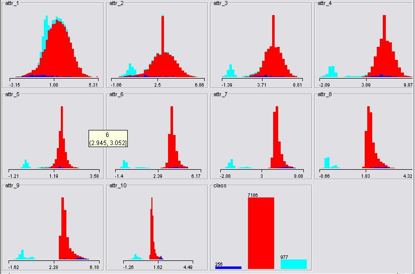
Preliminary Analysis:
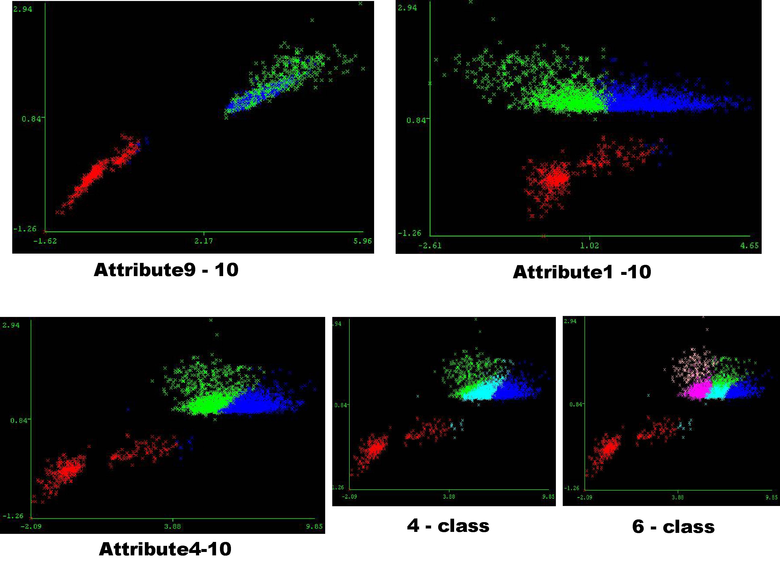
The two-class case seems very optimistic if we take a look at the graph of attributes plotted with respect to the "class" below:
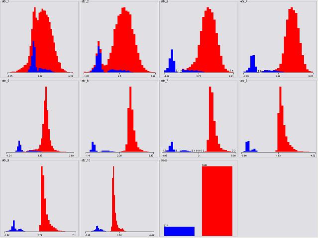
Attribute 7, 8, 9, and 10 separate the two classes completely, which means any of the attribute can be used to give a promised mining outcome. It is thus of less interest here to be further discussed.
The three-class case is unfortunately and fortunately not as simple as the two-class case. The plots of attributes demonstrate the difficulties.
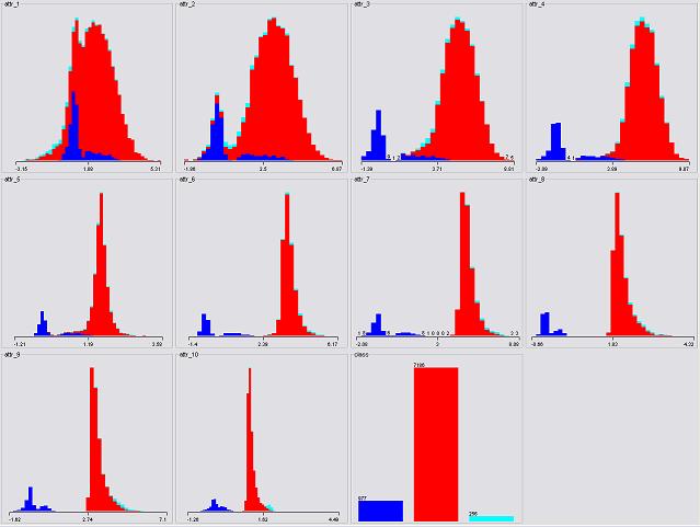
The main problem is the class "2" and "3" (i.e. red and light blue in the graph) as hardly an attribute can clearly separate them. And above all, attribute 10 is probably the most useful one in three-class case.
Some Results:
The two-class case is trivial, both techniques can guarantee the 100% correctness from mining. This can be seen clearly through the rule output by PRISM and DecisionTable (i.e. rule based systems):
Rules:
================================
attr_7 class
================================
'(-inf-3.047]' 1
'(3.047-inf)'
2
================================
Note that Weka probably run the algorithm sequentially through all attributes so attribute 7 is picked up first.
The three-class case can be directly mined by the two techniques (need to discritize attributes when using PRISM). The confusion matrices are listed in the table:
| BayesNet - 95.2497% | DecisionTable - 98.9521% | PRISM - 98.7426% | |||||||
| Class = > | a | b | c | a | b | c | a | b | c |
| a = 1 | 330 | 0 | 0 | 330 | 0 | 0 | 330 | 0 | 0 |
| b = 2 | 0 | 2328 | 126 | 0 | 2438 | 16 | 0 | 2437 | 11 |
| c = 3 | 0 | 10 | 69 | 0 | 14 | 65 | 0 | 17 | 60 |
DecisionTable uses an attribute set of {1,4,7,10}. PRISM uses all attributes but based on the information gain to rank the importance.
The information gain ranking is: 10, 9, 7, 8, 6, 4, 5, 3, 2, 1 (based on attribute sequence).
Other results are available in the Preliminary Analysis report [pdf].
Mining Results [pdf]
Visualization through Clustering
Some interesting information can be gained with clustering the dataset without predefined knowledge (i.e. class). The following plots show different clustering results from applying the k-mean algorithm using Weka.
 (Click
for full size)
(Click
for full size)
Class 1 is generally clustered in red which is a very pleasant case. Class 2 and 3 are confusing from the cluster plots.
The parallel plot and scatter plot are also very interesting to see here. Both of them demonstrate some important properties of this dataset.
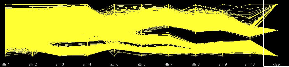 Parallel Plot
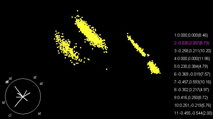 Scatter Plot
[To Index]
Dataset (Additional set with missing values from dataset #3)
Dataset Recovery
The most intuitive method to deal with the missing values is just to ignore them. The plots of attributes ignoring the missing values show very likely distributions from the previous dataset.
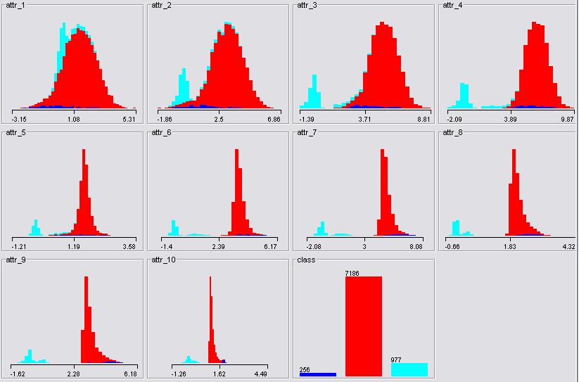
We also try to recover the missing values with the means. Following table lists the means of the 10 attributes subjected to classes (i.e., "4, 7, or 8") omitting the missing cells.
| Class/Mean | attr_1 | attr_2 | attr_3 | attr_4 | attr_5 | attr_6 | attr_7 | attr_8 | attr_9 | attr_10 | Total Sample |
| 4 | -0.098 | 1.317 | 4.051 | 5.958 | 1.475 | 4.147 | 6.047 | 2.657 | 4.542 | 1.888 | 256 |
| 7 | 1.498 | 3.081 | 5.198 | 6.370 | 1.594 | 3.701 | 4.871 | 2.108 | 3.277 | 1.170 | 7186 |
| 8 | 0.559 | 0.478 | 0.325 | 0.150 | -0.060 | -0.200 | -0.367 | -0.145 | -0.314 | -0.169 | 976 |
The process is then straight forward replacing missing values with the mean values in respect to the class and attribute number.
The plots of attributes after recovery is given below:
The parallel plot gives basically a same graph.
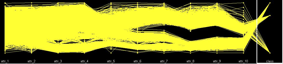 Parallel Plot
Note that there is a difference caused by sorting respecting to the class number.
General Result [pdf]
The recovered dataset with the means in general helps the Bayes methods to classify the dwarfs, but kind of misleading for the rule base systems.
The standard derivation table for each attribute after two preprocessing methods somehow states the point.
| Method | Class | attr_1 | attr_2 | attr_3 | attr_4 | attr_5 | attr_6 | attr_7 | attr_8 | attr_9 | attr10 |
| Ignore | 4 | 1.216 | 1.250 | 1.164 | 1.068 | 0.773 | 0.707 | 0.717 | 0.446 | 0.568 | 0.374 |
| Replace | 4 | 1.216 | 1.188 | 1.105 | 0.999 | 0.734 | 0.692 | 0.699 | 0.439 | 0.553 | 0.365 |
| Ignore | 7 | 1.082 | 1.120 | 1.048 | 1.020 | 0.278 | 0.333 | 0.431 | 0.267 | 0.398 | 0.158 |
| Replace | 7 | 1.081 | 1.056 | 0.994 | 0.975 | 0.267 | 0.321 | 0.418 | 0.260 | 0.388 | 0.154 |
| Ignore | 8 | 0.699 | 1.151 | 1.312 | 1.493 | 0.457 | 0.657 | 0.850 | 0.201 | 0.408 | 0.240 |
| Replace | 8 | 0.699 | 1.114 | 1.294 | 1.475 | 0.453 | 0.652 | 0.845 | 0.200 | 0.405 | 0.238 |
[To Index]
Weka Tutorial (Ulrike Sattler's introduction) - It is the best tutorial I could find online, but it is still somehow not that useful.
Weka Explorer Guide (University of Waikato) - I downloaded it from somewhere. Not for the newest version, but useable.
Weka Java Class Document (University of Waikato) - Java style documents for every class in the .jar of the package.
MatLab Introduction Tutorial (UF Mathematics) - I commonly refer to find commands.
The Pattern Classification Toolbox - Nice toolbox to visualize Bayes Classifiers. [Computer Manual in MATLAB to accompany Pattern Classification (by David D. Stork and Elad Yom-Tov)]
[To Index]